How to Train Your First Neural Network as a Developer
So you want to train your first image classifier, but don’t know where to start? We’ve got you covered.
So, you’ve heard neural networks are cool, but how do you get started? It’s easy for data scientists and machine learning engineers, but can a software developer like you train a neural network without prior knowledge? The answer is yes, and you’d be surprised with the amount of code required.
Today you’ll train and evaluate an image-based neural network for classifying handwritten digits. No prior machine learning knowledge is assumed — just the fundamental programming skills. You’ll do the coding in Python. It’s fine if you haven’t used the language before, as it’s easy to pick up if you’re coming from a different one.
We’ll write the code on Google Colab — a free online environment that lets you write Python code in a notebook format. More advanced users can work in their environments, but we assume you are a complete beginner to Python and machine learning.
Without much ado, let’s dive straight in.
Setting up the Environment
First things first — open up Google Colab. You should see a modal window like the one below if this is your first time:

Image 1 - Google Colab welcome page
From here, click on the blue New notebook button at the bottom right corner. You’ll be presented with a blank notebook in a matter of seconds:

Image 2 - Blank Google Colab notebook
You could change the runtime type to GPU by clicking on Runtime - Change runtime type - GPU, as neural networks train faster on GPU. The dataset you’ll use today isn’t resource-intensive, so you’ll be fine on the CPU. The model will train significantly faster on GPU, so keep that in mind.
Introduction to the MNIST dataset
The “Hello World” of deep learning is the MNIST dataset. It contains 60,000 images of handwritten digits (from 0 to 9), 6,000 for each distinct number. The best part is — it’s built into the deep learning library we’ll use today — TensorFlow — and is already split into training and testing sets.
Note: Training set is a set of images you’ll train the model on, and the test set is a separate set the model never sees during training. It’s used only for evaluation.
First things first — let’s import the libraries needed to follow along. You’ll need Numpy (fast mathematical operations for Python) and Keras (a high-level TensorFlow API for building models):
import numpy as np
from tensorflow import keras
from tensorflow.keras import layers
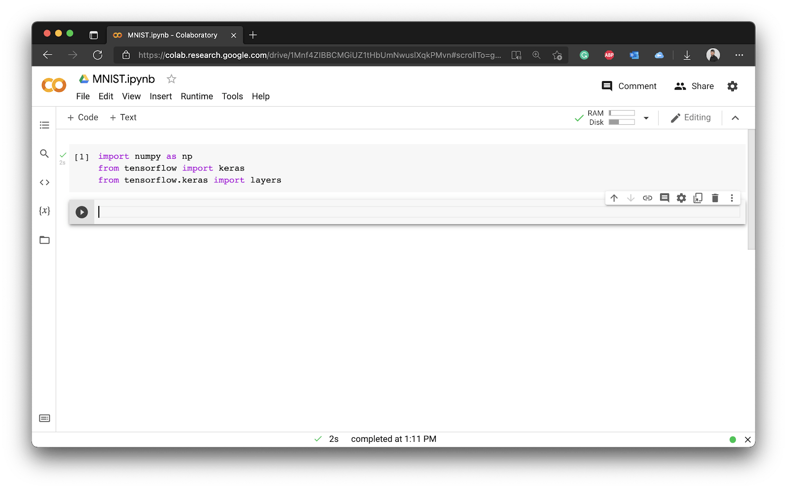
Image 3 - Library imports
Next, you can load in the MNIST dataset itself. It’s built into Keras and returns four elements — training images, training labels, testing images, and testing labels.
Note: In machine learning, features (images) are usually denoted with a capital X, while the labels (target) are denoted with a lowercase y.
You’ll have two additional variables, the first one for the number of classes (distinct numbers), and the other for the shape of a single image. Each image in the MNIST dataset is 28 pixels wide and tall, and has a single color channel (grayscale). For that reason the shape is (28, 28, 1):
(X_train, y_train), (X_test, y_test) = keras.datasets.mnist.load_data()
num_classes = 10
input_shape = (28, 28, 1)
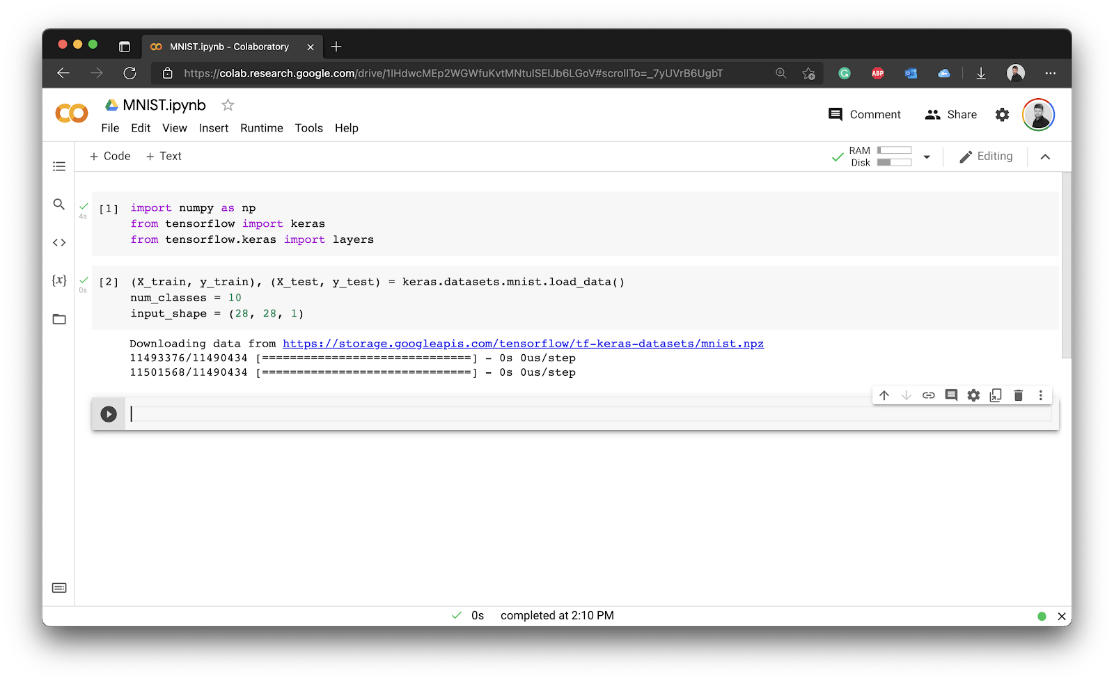
Image 4 - Loading the MNIST dataset
You can see how Keras automatically downloads the dataset for you. It’s now loaded, but how can you verify it actually contains images? The answer is simple — by visualizing one.
This step is entirely optional, so feel free to skip it. If you’re following along, import the Matplotlib library, print the first value of the y_train array, and use the imshow() function from Matplotlib to visualize the first value of X_train:
import matplotlib.pyplot as plt
print(y_train[0])
plt.imshow(X_train[0], cmap='gray');
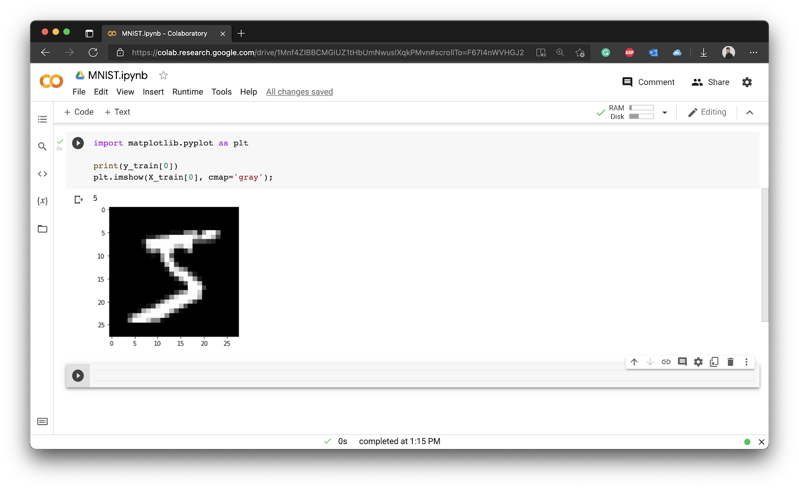
Image 5 - First digit of the MNIST training set
Note: X_train contains a list of matrices (2D arrays), each having 28 elements in both directions. These represent pixel values that you can easily visualize. On the other hand, y_train is a 1D array of labels, each showing the actual digit on the corresponding image.
You have now verified that the dataset indeed contains the images, so what’s next? There’s still one step to do before training, and that’s data preprocessing.
Preprocessing the MNIST dataset
The pixel values in a grayscale image range from 0 (black) to 255 (white). Neural network prefers a range between 0 and 1. You can convert the datasets from integer to float and divide the whole thing by 255:
X_train = X_train.astype('float32') / 255.0
X_test = X_test.astype('float32') / 255.0
The neural network won’t like that the image is missing color channel information. The images are in grayscale, which means they only have a single color channel, and that info was omitted by Keras. You’ll have to use the expand_dims() function from Numpy to add the missing color channel number:
X_train = np.expand_dims(X_train, -1)
X_test = np.expand_dims(X_test, -1)
That’s all with regards to the features. The shape of X_train should now be (60000, 28, 28, 1), indicating 60,000 images, each 28 pixels tall, 28 pixels wide, with a single color channel. You’ll see similar values for X_test, the only difference being the number of images:
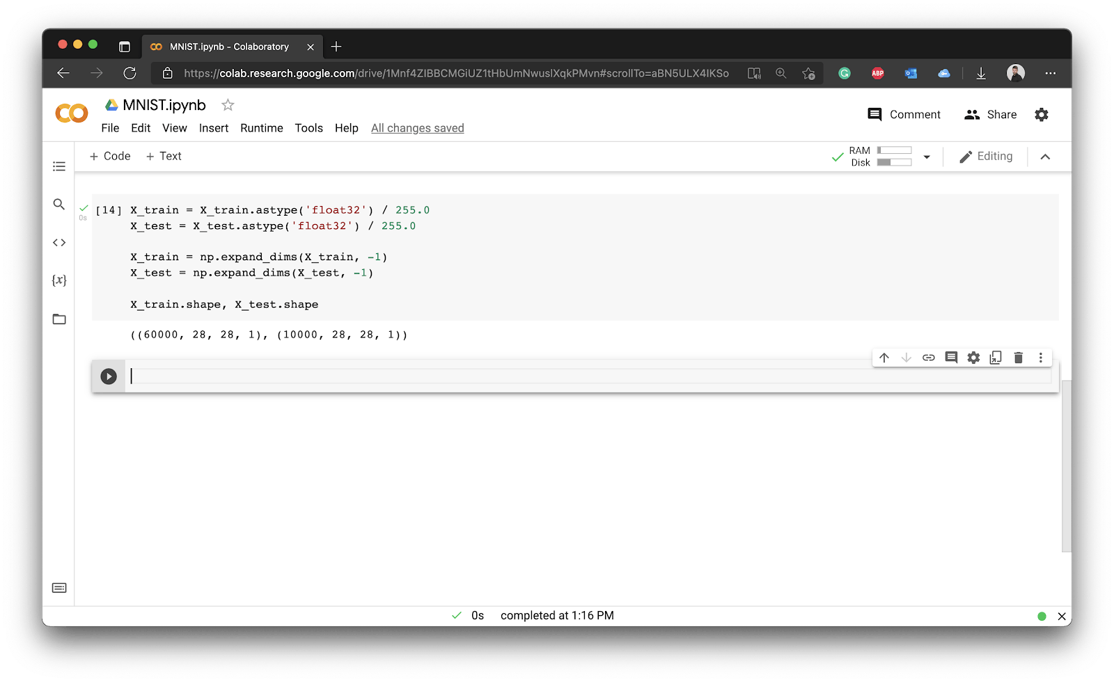
Image 6 - Preprocessing input features
Onto the target variable now. By default, it’s a 1D array containing labels. Neural networks want a one-hot-encoded representation, meaning each digit label must be converted into an array where all values except for the one are zeros. In our example, this means that the value of the array will be 1 at the index position which represents the image class:
y_train = keras.utils.to_categorical(y_train, num_classes)
y_test = keras.utils.to_categorical(y_test, num_classes)
y_train[0]
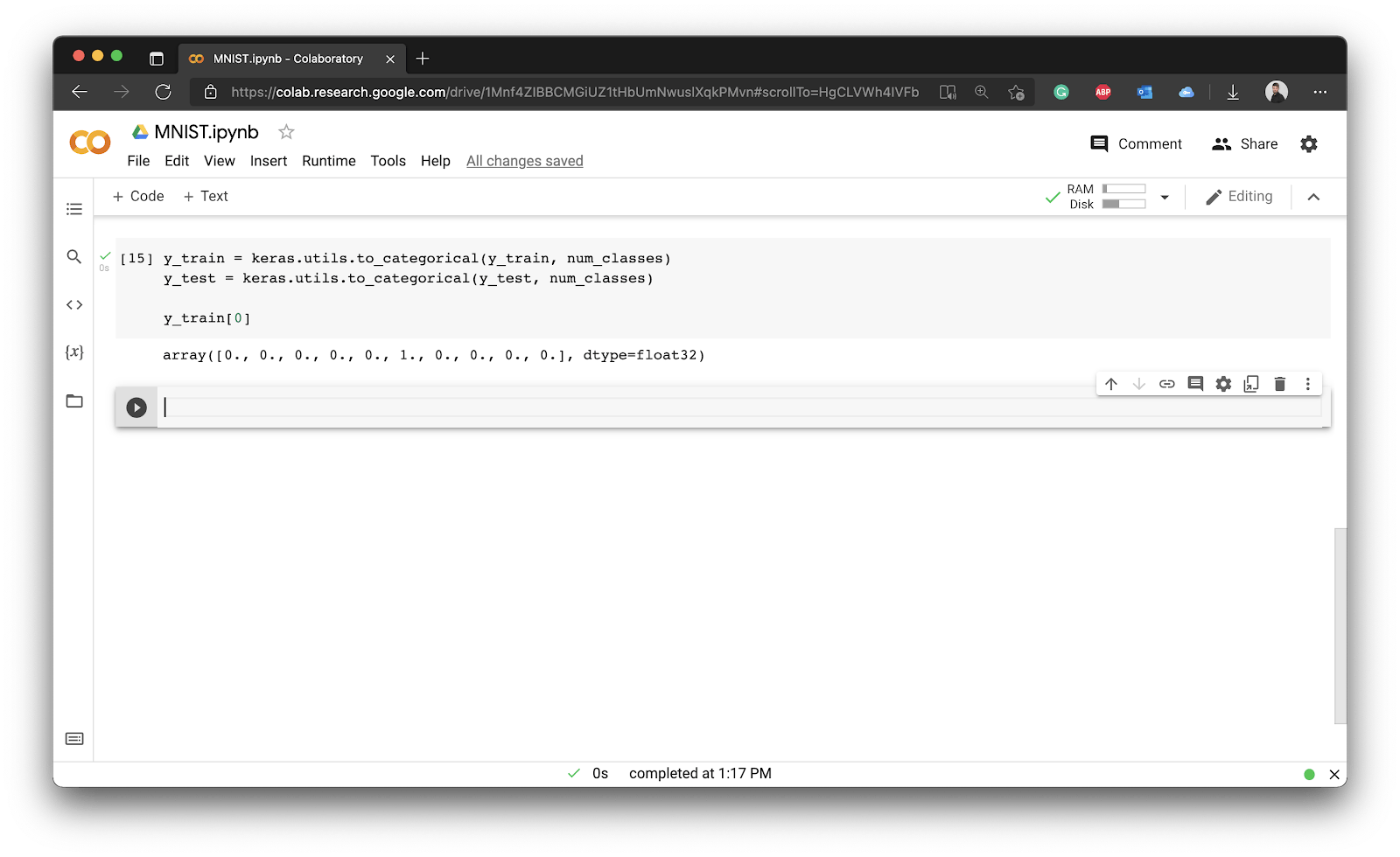
Image 7 - Preprocessing the target variable
Basically, each digit was converted into an array of 10 elements. The first array element represents if the corresponding image represents a digit zero, and so on. We have the value of 1 at the 6th index position, because the first training image represents a digit five.
And that’s all you need to start training the model!
Training a Convolutional Model
Wait, what is a convolutional model? Put simply, it’s a special type of neural network used in image classification. These networks have one or more convolutional layers, and their task is to extract features from images. It makes more sense to “learn” what makes number 0 a number 0 than to learn hardcoded pixel positions.
Convolutional layers are usually followed by a pooling layer. Its task is to reduce the output size by keeping what’s relevant. For example, a max pooling layer with a pool size of two will get rid of half the pixels. It keeps only the pixels with the highest values, which are the most relevant ones.
After a layer of convolution and pooling comes the flattening layer. It’s the simplest one by far — it turns the incoming N-dimensional input into a 1D array. It’s followed by a dropout layer, which serves as a regularizer. Neural networks tend to overfit (learn the training data too well), and a dropout layer will delete some percentage of neurons and their connections to avoid that behavior. A dropout rate of 0.5 means 50% of neurons and their connections will be removed.
Finally, we have an output dense layer. It will have 10 neurons (1 for each digit class), activated through a softmax function. This function turns the input values into probabilities, so you know what’s the probability of an image belonging to every digit class.
Sounds complicated? Well, it’s only a couple of lines of code:
model = keras.Sequential([
keras.Input(shape=input_shape),
layers.Conv2D(32, kernel_size=(3, 3), activation='relu'),
layers.MaxPooling2D(pool_size=(2, 2)),
layers.Flatten(),
layers.Dropout(0.5),
layers.Dense(num_classes, activation='softmax'),
])
model.summary()
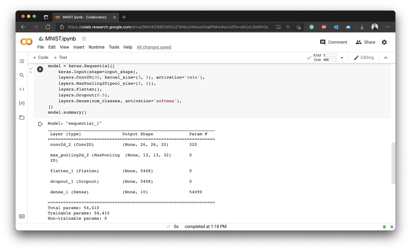
Image 8 - Convolutional model
Our neural network model has 54,410 tweakable parameters. This means a neural network has 54,410 little knobs it can adjust to give you the optimal model. That’s not a lot by today’s standards.
The next step is to compile the model. You’ll have to specify the value for loss, optimizer, and metrics. Don’t worry too much about these. The loss essentially means how the model is tracking error, the optimizer tells the model which method to use to adjust the knobs in the networks, and metrics represent a list of, well, metrics evaluated during training. The most common one is accuracy:
model.compile(
loss='categorical_crossentropy',
optimizer='adam',
metrics=['accuracy']
)
Finally, let’s train the model. During training, the model will see 128 images at once (batch_size) and will train for 10 epochs — the total number of runs through the entire dataset. You’ll train the model on X_train and y_train subsets, and from these, you’ll extract 10% for validation during training. It’s yet another separate subset used during training for an unbiased performance report:
model.fit(
X_train,
y_train,
batch_size=128,
epochs=10,
validation_split=0.1
)
The model will start training after you run this cell:
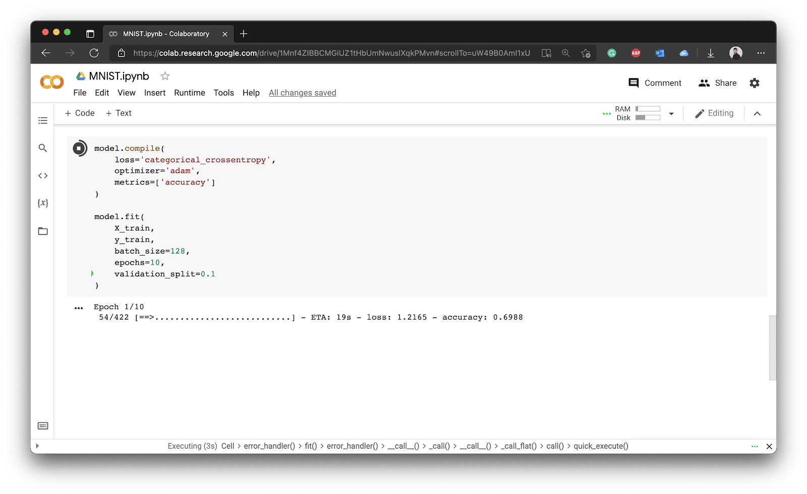
Image 9 - Model training (1)
You can see that it takes approximately 20 seconds per epoch, which is good enough for today. You’d see a significant decrease if you were to use a GPU environment instead. Why don’t you try it out?
Here’s what you should see after the training finishes:
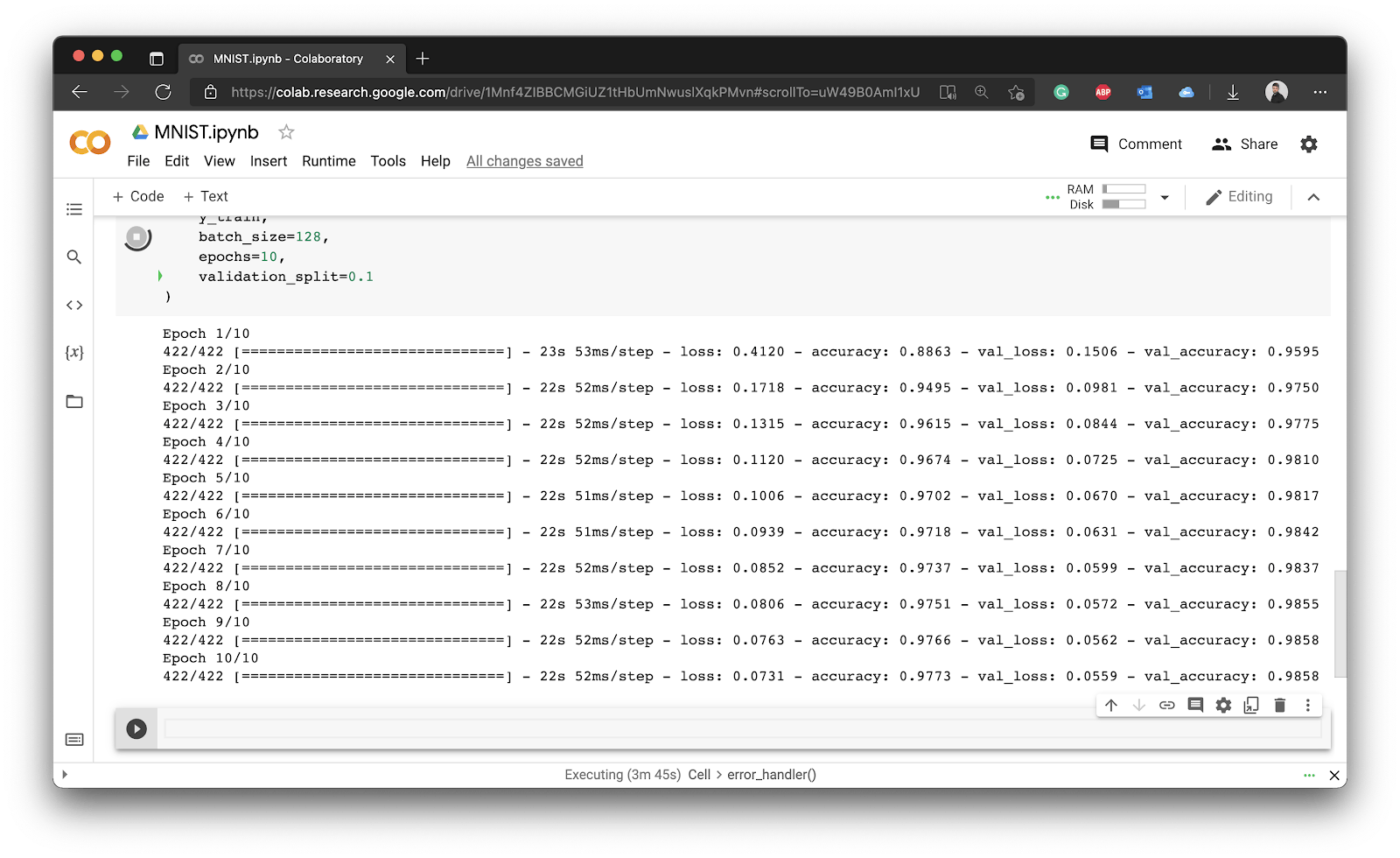
Image 10 - Model training (2)
After 10 epochs, we got 97,73% accuracy on the training set, and 98,58% accuracy on the validation set. For example, this means that the model on average classifies correctly 98,58 out of 10,000 images. Not too bad for your first neural network.
Finally, let’s explore how you can evaluate the model on the test set.
Evaluating Neural Network Models
After training, it’s a common practice to use the model to make predictions on the test set. Remember — you have it stored in X_test and y_test.
You can use the evaluate() function of your model to, well, evaluate it. The verbose=0 means nothing will be printed to the console during evaluation. You can then access the results of evaluation by indexing it — the first value represents the test loss, and the second one the test accuracy:
score = model.evaluate(X_test, y_test, verbose=0)
print('Test loss:', score[0])
print('Test accuracy:', score[1])
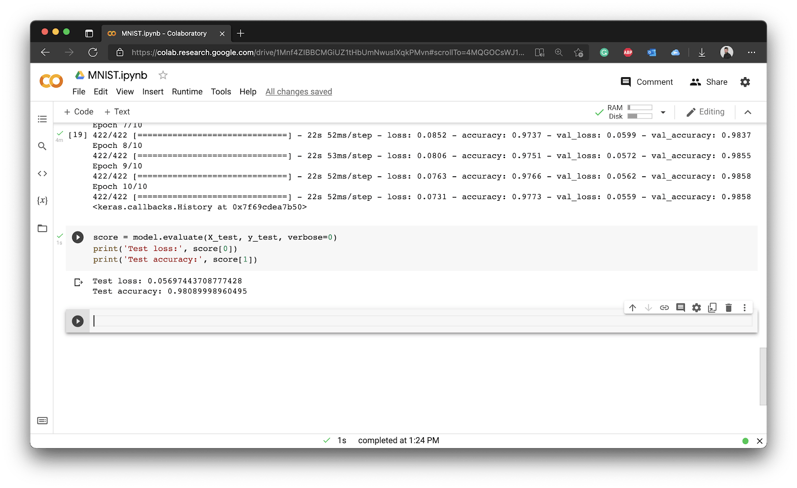
To summarize, we got 98,09% accuracy on the test set. These are astonishing results, but you can still improve.
Conclusion
And there you have it — your first neural network for classifying handwritten image data. You have to admit — it wasn’t a whole lot of work. It would take around 20 lines of code if you were to count it.
Training neural networks is actually this easy, code-wise. The hardest thing about it is understanding what to use when, and adequately preparing the data. You won’t always have the luxury of using a built-in dataset.
If you want to take your model to new heights, here’s a couple of homework assignments:
- Try tweaking the number of filters in the convolutional layer — how does it affect the accuracy?
- Try adding another convolutional and pooling layer combination — does it have any impact on the performance? Can you reason why?
- Switch to a GPU environment in Google Colab — how does it affect the training time? What’s the fundamental difference between a CPU and a GPU?
Overall, you did a lot of work today. There’s still a lot of ground to cover, but take it one step at a time.
